Provenarium User Guide

Before you start

Use an individual account and the browser approved by your organization. Provenarium’s release testing uses a specified Chromium version; check the release documentation when qualifying a browser for your laboratory.

Have access to your email inbox if you are creating an account or joining a Team. Use the workspace address supplied by your organization or the Try the workspace link on this site. The public demonstration workspace contains synthetic records and resets; it is not a place to retain your laboratory work.

Create an account or sign in

1. On the sign-in page, choose Create account for a new account. Enter Your name, Email, Password and Confirm password, then choose Create workspace. The password must contain at least eight characters. Alternatively, use Continue with Google with your intended account.
2. For an existing email/password account, choose Sign in, enter Email and Password, and choose Continue to workspace. For an existing Google account, choose Continue with Google.
3. Use Current workspace to select Personal or the named Team. Check the displayed name before uploading a file or creating work. A different Team is a different set of records and permissions.
4. When finished, wait for any draft save to finish, then choose Sign out. Do not leave a shared computer signed in.

Accept a Team invitation

Invitations are single-use and expire after seven days. A wrong-account, expired or already-used invitation cannot be repaired by sharing an account; ask the owner for a correct invitation.

1. Open the invitation link from the Team owner. Sign in or create an account using exactly the invited email address. The invitation flow uses Continue to invitation.
2. If asked to verify your email, choose Send verification email, follow the email link, and return to the invitation. Follow the displayed check to confirm verification.
3. Check the Team and offered role, choose Accept and join Team, then Open your workspace. Select the Team in Current workspace and check that it appears as expected.

Recognize the workspace and role

A review assignment, rather than the role’s name, determines who can decide a particular review. Contact Provenarium for supplier documentation to support your laboratory’s validation work.

When access is not what you expect

If the Team is unavailable, select Personal to continue separate free manual work or contact the Team owner. Do not move controlled work into Personal to bypass Team access.

If the wrong records or no records appear, first check Current workspace, then the page filters. Signing in with a second account can create a different Personal workspace; use the intended account.

For lost account access, use your identity provider’s recovery process or contact Provenarium. The app does not currently offer a separate password-reset control on its sign-in page.

Prepare the file

Keep the authoritative instrument export. Assay files may be UTF-8 CSV, TSV or TXT, or a supported static XLSX workbook, up to 15 MiB. Limits include 10,000 rows, 1,024 columns and 250,000 rectangular cells; a workbook shares the cell limit across its supported worksheets. Select a 96-well or 384-well rectangle.

CSV permits comma or semicolon, TSV uses tab, and TXT permits comma, semicolon, tab or pipe. Select the delimiter yourself if the columns do not appear as expected.

Provenarium reads saved values from supported XLSX worksheets; it does not recalculate formulas. Save calculated values in Excel before uploading and check the imported measurements and units. Legacy XLS files, macros, external links and unsupported workbook objects are rejected.

You can add PDF and DOCX documents as supporting information when planning with assistance. Upload the measurements separately as an assay data file. Supporting files are limited to 5 MiB each; a message explains if any content cannot be read. Check formula results in supporting spreadsheets against the original workbook.

Select the source and exact plate region

1. In manual setup, use Choose file on Import plate measurements. Check the displayed filename. If the file is rejected, correct the stated encoding, format, size or workbook problem and select it again.
2. Under Data selection, inspect the Sheet and Delimiter when available. Select the worksheet that contains the intended measurements; different sheets can contain different experiments.
3. Check Plate size, Top-left cell and Selected range. The selected rectangle must contain just the measurement grid, not row/column headings or notes. Use the worksheet preview and its Previous/Next rows or columns controls if the region is outside the visible window.
4. If shown, choose Confirm exact range after inspecting it. Continue when the plate range is ready. For example, source cells B6:M13 become plate wells A1:H12: a source cell address and a plate well name are not the same coordinate.

Assign the used wells

1. On Map the plate, inspect the preparation list and names. Use + Add sample for another preparation and select the appropriate role. Relative potency needs a reference and test preparations; concentration work uses standards, unknowns, optional quality controls and blanks.
2. Select a measured well. In its editor, set Sample, Dilution level and Replicate to match the physical experiment. Repeat for each used well. The same preparation and level may have multiple replicates; a new sample name alone does not map any wells.
3. A template can provide a starting map, but inspect every assignment before continuing. Do not apply a template over a custom map unless you intend to replace those assignments.
4. Keep absent observations distinct from zero. Empty/missing wells are not measured zero responses and cannot be used as valid observations. Leave unused measurements unassigned.
5. For a scientifically justified manual exclusion, select the mapped well, use Exclude from fit and enter the required reason. Check the recorded exclusions; do not remove a result simply to improve fit or suitability.
6. Continue to Define the dilution series and inspect Mapped observations. Check preparation, response, level, replicate and calculated concentration together before choosing the model.

Resolve a wrong map or missing value

If measurements look shifted, return with Back and check the selected source region before changing scientific settings. If only a sample, level or replicate is wrong, correct that assignment in Map the plate and review Mapped observations again.

An invalid or insufficient design must be corrected before Run. In routine mode the recipe is locked: if the new plate does not match the approved layout, stop and use a compatible source or the controlled Method revision process.

Before continuing, check that every well you intend to use has the correct preparation, level and replicate assignment.

Before you start

Have measured assay data and a justified procedure for mapping, units, dilution, model and suitability. If you want to practice first, use one of the synthetic walkthroughs. The example settings are not recommendations for an unknown assay.

Work through the configuration

1. Open New analysis. Select Relative potency to compare preparations with a reference, or Concentration determination to estimate unknown concentrations from standards. Choose Configure manually.
2. Use Choose file, check Data selection, and Continue to Map the plate. Assign used wells, levels and replicates as described in Import and map assay data.
3. Continue to Define the dilution series. Set Concentration unit. For relative potency, set Initial concentration and Dilution factor for each preparation and inspect the mapped levels. For concentration work, define the standard concentrations, unknown and quality-control dilution factors, replicate treatment and expected QC concentration when applicable. Inspect Mapped observations for the values that will actually be used.
4. Continue to Model. Choose the exact model card and inspect its settings. Set scientifically justified transformations, weighting, response units, orientation and any model-specific choices that are shown. Options vary by family and model; do not select a model solely because its curve looks better.
5. Check any configured suitability rules and their limits. Add only criteria specified for your use. No user-defined criteria does not mean that an assay has been validated or automatically accepted.
6. Use Back and Continue to inspect the full configuration. Wait for Draft saved and resolve validation messages before Run analysis. Check the filename and settings when you reopen a draft.

Understand saved and unsaved work

The editor saves drafts automatically; there is no separate final Save draft step. Saving draft… or Unsaved changes · saving shortly means your latest changes are still being saved. Draft saved confirms the current saved draft.

Keep or bookmark the draft address after it has saved. Reopen it in the same account and workspace. Workspace selection preserves its own unfinished work; check that the reopened filename and settings match the task you intended to continue.

Configure manually from assisted setup begins separate manual work. The conversation and its saved files remain in the assisted setup; unsent text and unuploaded files are not transferred.

Resolve an invalid or conflicting draft

If a required value is missing or invalid, correct the named field and review the affected mapped observations. Do not substitute zero for unknown units or missing concentrations.

If Draft changed elsewhere appears, another tab or session has changed the saved draft. Inspect the displayed problem and preserve any needed local notes before using Discard local edits and reload saved draft. Check the reloaded values before continuing.

If Draft save failed appears, use the displayed retry or recovery control and confirm Draft saved. Keep the tab open until your changes have saved.

Before you start

Know what you want to determine or compare. You can discuss the objective before choosing a model or adding data. To propose a configuration, you will need assay measurements and the information that gives them meaning: samples, standards or reference, concentrations, units, dilutions and replicates.

Use only material your organization permits you to share with the assistance service. Have the relevant procedure or supporting documentation available to check the proposed settings.

Assay data can be CSV, TSV, TXT or a supported static XLSX workbook. Supporting PDF or DOCX documents provide context, not measured assay data. PDF support uses extracted text and tables; it does not perform OCR or let the assistant visually interpret pages. Inspect the original PDF yourself when needed.

Prepare a configuration

1. Select the intended Team workspace and open New analysis, then select Start conversation. Under Plan your analysis, enter your objective in Message and select Send. For example: “I want to compare the potency of my test samples with a reference.” If an existing setup opens, check that its objective and inputs belong to the work you intend to continue.
2. Use Message and Send to discuss the task, supply missing facts or ask about supported approaches. Read the response. Send continues the conversation. It does not change your saved settings or run the analysis.
3. Open Add files and supporting context. Under What are you adding?, choose Assay data, select the Assay data file and select Add input. Check that the file appears in the added inputs. Select the appropriate supporting input type to add documents or notes in the same way; confirm a Delimiter for supporting tabular files if requested. Selecting a file alone does not add it.
4. In Current analysis brief, use Choose analysis family and then Confirm analysis family if the family is still unselected. Choose Relative potency to compare a test preparation with a reference, or Concentration determination to estimate unknown concentrations from a calibration curve. Discussion can help you decide; you confirm the family.
5. Finish adding selected inputs and save or discard any objective changes. Send or clear any unsent Message. Select Propose configuration when the family is confirmed and assay data is present. The assistant prepares and saves a draft for you to review.
6. If a question appears, supply the missing facts and select Answer and continue preparation. That answer continues the requested preparation and may save the draft. To discuss alternatives or change inputs first, select Pause preparation. Do not invent missing concentrations, units or procedure details just to proceed.
7. When the editor opens, inspect the saved configuration and its evidence. Use Back and Continue to review source selection, mapping, model, units, dilutions, transforms, weighting and suitability settings. Check cited material and assumptions against your actual procedure. A saved proposal is ready for your review; it is not an approved scientific method.

Recognize the result

When the proposal is ready, it opens in the analysis editor. You can check and edit the settings, read their sources and see whether your changes have saved. The analysis has not run yet.

You can edit manually or describe a change and select Update configuration in the editor. Send still requests discussion. Review the resulting settings and any unsaved edits before choosing Run analysis. Running, interpreting results and retrieving reports are separate tasks.

Change the objective or family

Before a proposal is saved, edit Analysis objective and choose Save objective, or choose Discard objective changes. Saving an objective change keeps files and context but clears earlier proposed settings and questions.

To change family, use Current analysis brief: select Change family, choose New analysis family, then select Change analysis family. Your conversation and files remain available. Earlier proposed settings and pending questions are cleared, so request Propose configuration again. A previously saved analysis and its results stay unchanged; the new proposal creates a separate draft.

Recover when you cannot continue

If Propose configuration is unavailable, confirm the family, add assay data, finish or clear selected inputs, save or discard objective edits, and send or clear your message. An active preparation must be answered, resumed or paused before starting another.

If the response is interrupted, use Check same request when shown. This checks whether your original request finished and saved a draft. Use Open saved analysis when offered. Do not repeatedly submit a new proposal to recover an uncertain request. Other displayed recovery controls include Retry saved request and Reload conversation; follow the message beside them.

If a file cannot be read or used, read the message, correct the problem and add it again. For a scanned PDF, supply an appropriate text-based source or the necessary facts with a clear basis. Do not assume unreadable evidence informed the proposal.

If assistance is unavailable, check that you are in an active Team with a role that can create drafts. Contact the Team owner for access problems. To proceed manually, confirm a family and choose Configure manually. Manual setup starts separately; saved conversation and files stay in the assisted setup, and unsaved text or unuploaded files are not transferred.

If the draft changes while an update is being prepared, review the latest saved settings and decide which edits to keep before requesting another update.

What to do next

Review the draft against your procedure before running it. Use the walkthroughs below to practice the same inputs with manual setup or assistance. For help with your workflow or documentation, contact Provenarium.

Before you start

Open your saved analysis after Propose configuration succeeds. Have your procedure and the original supporting material available. Read the cited sources to check that the proposed settings reflect your procedure.

Inspect settings and their evidence

1. Use Back and Continue to visit each editor step. Read Current saved draft or Pending local edits in Configuration help before relying on the explanation.
2. Open Explanation and sources for this step. Check what the source actually supplied, what was recommended, and any assumptions or unanswered facts. These details describe the saved revision, not unsaved screen edits.
3. Select a cited evidence marker to inspect the quoted passage, cells or document context. Check the surrounding material and source identity. A citation to older guidance shows the version used for that proposal.
4. For PDF evidence, choose View original page for the offered page. Use Actual size or Fit page to inspect it. The assistant reads extracted text and tables, not page images. Inspect figures and scanned content yourself.
5. After you edit a proposal, Original proposal explanation (revision 1) still describes the original settings. Use Refresh help when the editor says its context has changed.

Ask a question or change the settings

1. For a question only, enter Message about this configuration and choose Send. The response can discuss settings, including separately labelled local edits; it does not save changes.
2. For a change, first reconcile any pending local edits or save conflicts. Describe the intended change and its basis, then choose Update configuration. This asks the assistant to change and save the settings.
3. Answer any follow-up questions. When the update finishes, compare Setting, Before and After, then check the saved settings in the editor before choosing Run analysis.

Recover an interrupted or rejected update

Use Check same update when its result is uncertain. If offered, Resume reviewed update continues the update you were reviewing. Cancel update and keep draft stops it. Check the saved draft rather than assuming an interrupted response lost the save.

If the draft was changed in another tab or session, review the latest saved settings and decide which edits to keep before asking for another update.

Missing or unreadable evidence is a reason to supply better source material or correct the facts. Do not interpret a fluent explanation as a substitute for the required evidence.

Before you run

Confirm workspace, input, map, concentrations, model, settings, exclusions and criteria. Wait for Draft saved in development, or confirm the exact approved Method/version in routine mode. The analysis starts only when you choose Run analysis.

Run the analysis and review the results

1. Select Run analysis when the configuration is ready. Wait while the analysis is queued or processing. If the connection is interrupted, reopen this analysis to check its progress before starting another run.
2. When the completed analysis detail opens, check the analysis name, family/model, source and Method/version if present. The application retains the result and automatically generates its report. Completing development does not itself create a Method.
3. For relative potency, inspect Model adequacy and comparability and Suitability and manual exclusions; read each preparation’s potency and interval in the PDF report. For concentration, read Analysis summary and Concentration results for unknowns and quality controls, units, reportability and dilution-adjusted values. Open the detailed evidence to inspect standards, per-well values and exclusions.
4. Read any calculation errors or warnings and the results of the model’s required checks and your configured suitability criteria. Check each affected preparation or sample, not only the overall badge.
5. In the report area, select the required Report revision, choose Load PDF preview, inspect the saved report and then use Download PDF. Reopen the downloaded copy and confirm it is the intended result before filing it.

Distinguish the outcomes

If the result or report is unavailable

If the connection was interrupted, reopen the same analysis to check whether it finished. If only the report failed to open or download, try opening that report again; you do not need to rerun the analysis.

Completed analyses cannot be edited. To change the inputs or settings, create a linked development copy or start a new analysis. The original result remains available alongside the new work.

A PDF report supports your filing procedure; it is not a complete Team archive. Personal results can be reopened from their saved detail address even though the Team Analyses library is unavailable in Personal.

Get the synthetic inputs

This example uses a common-shape 4PL plate with eight levels and two measured replicates for each of three preparations. It should yield approximately 80% for Test alpha and 120% for Test beta. These are demonstration results, not customer qualification evidence or acceptance criteria for your assay.

Download the CSV below. Keep the setup note if you want to try the assisted alternative with the same measurements. All data and screenshot records are synthetic.

• Download relative-potency example CSV
• Download relative-potency setup note

Configure the example manually

1. Select your workspace. Open New analysis, choose Relative potency, then Configure manually. Choose file and select relative-potency-multi-preparation-4pl.csv.
2. Check comma-delimited text, the 96-well plate and source range B6:M13; Confirm exact range if prompted. Continue to Map the plate.
3. Choose Apply two-curve template before adding another sample. Choose + Add sample. Keep Reference standard and rename the two tests Test alpha and Test beta.
4. For every row A–H, select each well that needs changing and edit Sample and Replicate. Columns 1–2 are reference replicates 1–2, columns 3–4 are Test alpha replicates 1–2, and columns 5–6 are Test beta replicates 1–2. Specifically, change column 3 to Test alpha replicate 1, column 4 to replicate 2, and columns 5–6 to Test beta replicates 1–2. Keep the template’s row-based levels: A is level 1 through H as level 8.
5. Check 16 wells per preparation, 48 included measurements in total, no exclusions, and columns 7–12 unassigned. Continue to Define the dilution series. For each preparation, set Initial concentration to 128 ng/mL and Dilution factor to 2. The eight levels must be 128, 64, 32, 16, 8, 4, 2 and 1 ng/mL.
6. Continue to Model and select Common-shape 4PL. Check Dose transformation: Natural logarithm; Response transformation: Untransformed; Weighting: Unweighted. Keep the example’s fixed default reference assignment of 100 and no additional user suitability criteria. Review all settings and wait for Draft saved.

Use assistance with the same inputs

Use the map and settings above to check the proposal before running it. The assistant’s wording and questions may vary.

1. In a Team where you can develop analyses, begin a separate New analysis with Start conversation. Enter “Compare Test alpha and Test beta with Reference standard using common-shape 4PL and the supplied synthetic setup” in Message, then Send.
2. Add the same CSV as Assay data and relative-potency-context.txt as Supporting document using Add input for each. Confirm Relative potency in Current analysis brief.
3. Discuss any missing facts, then select Propose configuration. If asked for clarification, answer from the setup note. Inspect the saved draft against the map and settings above before running. Assistant wording may differ; compare the actual settings and cited evidence.

Run the analysis and save the report

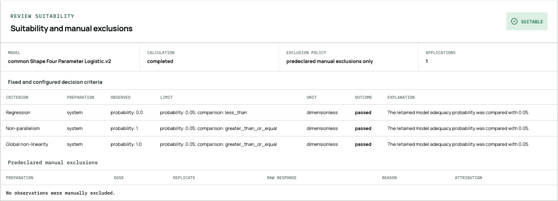
1. Choose Run analysis. When the completed detail opens, inspect Model adequacy and comparability and Suitability and manual exclusions.
2. Choose Load PDF preview. In the PDF report, check the separate Test alpha and Test beta results: approximately 80% and 120% respectively, with their intervals. For the unchanged synthetic recipe, the calculation and fixed suitability checks pass; no observations are excluded.
3. Use Download PDF, reopen it and check both preparations and the intended source before filing the copy. Keep the saved analysis address for reopening.

Extend the example through approval and routine use

1. As the result’s creator in a Team, enter a Method name such as Synthetic potency example and select Save as new Method draft. Open View Method draft and inspect the saved recipe and source report.
2. Select two qualified current Team members under Required approvers, enter a reason explaining this synthetic exercise and Submit for review. Each person uses their own account and assigned review.
3. Each approver opens Reviews, checks the exact Method version and evidence, enters Required decision reason and chooses Approve. Check the confirmation, confirm signing intent and complete Sign and approve or Continue with Google as displayed. After both decisions, check Approved · version 1.
4. Open that approved Method and choose Run approved Method. Enter an Analysis name, upload the same synthetic CSV to demonstrate reuse, confirm B6:M13 and inspect the locked map and settings with Continue. Choose Run analysis.
5. Check a new routine result linked to version 1. It should again show approximately 80% and 120%. Preview, download and reopen its own PDF report. Reusing synthetic measurements here demonstrates the workflow; real routine work uses a new assay source.

If the expected result does not appear

First check the map. The two-curve template originally assigns column 3 to the reference and columns 4–6 to one test; the three-preparation example requires the edits above. Confirm two replicates per preparation/level and an initial concentration of 128 for all three preparations.

If a unit is missing during assistance, provide the documented ng/mL dose unit and the setup note; do not guess from the file’s numeric values. If a calculation or suitability check fails, inspect it before using any numerical result. Do not remove observations simply to recover 80% or 120%.

Get the synthetic inputs

The plate contains six paired standard levels, two independent unknown measurements, a quality control and a blank. The unknown should be about 60.5 ng/mL after its ten-fold dilution correction, and the QC about 100 ng/mL. These are example results, not customer qualification evidence.

• Download concentration example CSV
• Download concentration setup note

Load and inspect the manual example

The editor numbers standard levels from the highest concentration down; the CSV places the pairs from low to high. Inspect the concentration associated with each well rather than assuming that level 1 means the leftmost pair.

1. Open New analysis, choose Concentration determination, then Configure manually. On Import plate measurements, choose Load example assay. This loads interpolation-linear.csv and its example configuration; it does not run it.
2. Confirm the 96-well source range A1:L8. Continue to Map the plate and inspect the assignments in the table below. Leave all other wells unassigned, even though the source contains numerical zeros there.
3. Continue to Define the dilution series. Check ng/mL, the six standard concentrations and reportable standard roles, ten-fold dilution factors for Unknown 1 and Quality control 1, and expected QC concentration 100 ng/mL. Standards are technical replicates within each level; the unknown and QC are independent replicates.
4. Continue to Model. Check Linear calibration, Untransformed concentration and response, Unweighted and increasing Curve orientation. Inspect the example’s minimum calibration R-squared criterion: 0.980 at three decision decimal places. Keep the example settings and no exclusions.
5. Check the displayed reportable calibration range of 1–32 ng/mL and wait for Draft saved. This range applies to the concentration interpolated on the curve; the sample’s dilution-adjusted concentration can be larger.

Prepare the same analysis with assistance

For a useful recovery exercise, discuss the unknown without giving its dilution factor and ask what is missing. Supply the documented factor 10 when requested. Do not assume the assistant can infer sample preparation from responses alone.

1. In a Team where you can develop analyses, start a separate conversation and Send: “Determine the unknown and quality-control concentrations using linear calibration and the supplied synthetic setup.”
2. Add the downloaded interpolation-linear.csv as Assay data and concentration-context.txt as Supporting document. Confirm Concentration determination, then select Propose configuration.
3. Use the setup note to answer any questions. Inspect the saved draft against the map, units, dilution factors, replicate treatment, model and criterion above. Request Update configuration or edit manually if a setting differs; review the saved state before Run.

Run the analysis and save the report

1. Choose Run analysis. Read Analysis summary and Concentration results on the completed detail. Expect Unknown 1 approximately 60.50 ng/mL (60.49–60.51 for this unchanged example) and QC approximately 100 ng/mL, with the displayed reportability and interval information.
2. Inspect calibration evidence, standards and per-well details. The unknown responses 12.0 and 12.2 correspond to about 6.0 and 6.1 ng/mL on the calibration curve before the ten-fold correction. The reported result combines the replicate estimates before rounding, so a calculation using rounded values may differ in the last displayed digit.
3. Read the suitability result and QC recovery. Then choose Load PDF preview, inspect the saved result and use Download PDF. Reopen the file and confirm the same source, model, units and result before filing.

If the result is missing or outside the expected range

Check A1:L8, the standard-pair concentrations, B1–B2 unknown assignments and dilution factor 10. If the result is about ten times too small, inspect the dilution factor before changing the model.

A sample outside the reportable calibration range is not automatically extrapolated. Review the displayed reason and follow your procedure for dilution or repeat measurement; do not convert an unavailable concentration to zero.

The blank is recorded, but its response is not automatically subtracted from the other measurements. Keep the example’s untransformed measurements unless a justified procedure specifies otherwise.

Before you start

Use a completed Team development analysis you own, with its saved report ready. Inspect its inputs, settings, results and suitability. To create a Team Method, the development analysis must have been run in that Team.

Choose qualified approvers according to your procedure. Any current Team member can be assigned; the Reviewer role alone does not grant authority over an unassigned review. Approval applies to an exact Method version, not the customer’s assay validation or a result report.

Create and submit the draft

1. Open the completed analysis. Under Save these settings as a Method, enter Method name and choose Save as new Method draft. If the analysis came from an existing Method version, verify that lineage and use Save as next draft version instead.
2. After Method draft created appears, choose View Method draft. Inspect the recipe and its source development analysis/report. Completing the analysis and creating this Method are separate actions.
3. In the Method draft, choose Required approvers and enter Reason. Check every selected person: all selected approvers must approve this exact version. Choose Submit for review.
4. Confirm In review with the intended version. The Method becomes available for routine use when all required approvers have signed.

Review and sign the exact version

1. As an assigned approver, select the correct Team and open Reviews or the relevant notification. Check Method to review, version, recipe and source evidence before deciding.
2. Enter Required decision reason. To return the work, choose Request changes; this closes the review without an approval signature.
3. To approve, choose Approve. In Confirm electronic signature, check the exact record, meaning Approved and your reason. Cancel if any item is wrong.
4. Confirm I intend to electronically sign this exact record with the meaning “Approved.” Complete password reauthentication if requested and choose Sign and approve; for Google, use Continue with Google when shown. Use your own account.
5. Check the recorded decision. Until every assigned person signs, the review still has pending decisions. After the last approval, confirm Approval complete and the Method’s Approved status/version.
6. Reopen the review history and signature details when needed. They identify signer, signing time, meaning, reason and the exact signed record. Only a completed signature records your approval.

Revise, reroute or retire

After changes are requested, return to the Method and use its development action (Start development analysis or Copy to development analysis as displayed). Complete the revised development result, then Save as next draft version. Review the new version; the previous result and decision remain available.

If assignments are wrong, an authorized review-routing user can choose Change required reviewers, select Reviewers for the new review, enter the required reason and Replace review. Cancel review ends the active attempt when appropriate. Check the replacement or cancellation before asking anyone to sign an old link.

An Owner or Admin can choose Retire for an approved Method, entering the required reason. A retired version remains historical evidence and cannot start a new routine run. Retirement does not alter its earlier analyses or signatures.

If you cannot create, decide or sign

A disabled Method action may mean you are in Personal, do not own the result, lack development permission or the saved report is not ready. Check your workspace and role, and confirm that the report is ready.

If Approve is missing, check the Team, active review, exact assignment and whether you already decided. A changed, cancelled or replaced review must be reopened at its current state.

If signing fails or expires, reread the error, reload the current review and check whether your decision was recorded before trying again. Do not treat reauthentication alone as a signed approval.

Before you start

Know the approved Method and version required by your procedure. Prepare new assay measurements with the layout, sample roles and units that its recipe expects. A routine run uses the saved recipe, not a fresh model choice.

Run the locked recipe

1. Open Methods, choose the intended Method and version, and check Approved. Select Run approved Method. You can also reach the Method library from New analysis using Choose a method.
2. Confirm the Approved Method name/version shown in the workflow. Enter Analysis name so the new run can be identified later.
3. Use Choose file for the new measurements, confirm the worksheet/region and Continue through the map, dilutions and model. Inspect the locked settings and ensure the new plate matches them.
4. Use Run analysis when ready. Watch the existing operation until the saved result opens, then inspect the calculation, suitability, exclusions, source and Method/version.
5. Select Load PDF preview and Download PDF for that completed run. Confirm the report belongs to the new data and exact Method version before filing it.

Recognize the routine result

The new analysis records the source file, results and report, together with the approved Method version used. It does not replace the development analysis or an earlier routine run. A passing calculation or suitability badge is not automatic sample release.

If the Method or data is incompatible

Draft, in-review and retired versions cannot start new routine work. Select the correct approved version; if none is suitable, use the controlled development and review process.

If a saved Method is incompatible with the current product, use the offered action to copy it for development, then review a new version. Do not alter the old recipe or describe an unapproved development result as a controlled routine run.

If the file or plate layout is wrong, stop and select the correct compatible source. Routine settings are deliberately locked; moving to development is not an override of an approved Method.

Choose the comparison question

Know which preparations, result quantities and Method versions you intend to compare. Use the comparison or trend to inform your investigation; interpret any differences alongside your assay knowledge and laboratory procedure.

Compare two analyses

If a candidate is not offered or the comparison is rejected as incompatible, check family/model and result availability. Relative-potency and concentration analyses cannot be made equivalent by forcing a comparison.

1. Open Analyses. Use Search and Run type as needed, then Apply filters. Load more analyses if the desired records are not yet loaded.
2. Select Baseline result, then a compatible Candidate result. Choose Compare results.
3. Check the named baseline and candidate and compare their settings and preparation results. Follow the source analysis links to inspect the full result and report before drawing a conclusion.

Inspect a Method’s routine results over time

1. Open Trending and select Method and Method version. Use the fixed approved or retired version relevant to the historical question; changing the version changes the dataset.
2. Select an available metric, such as Relative potency, and Sample when required. Set From date and Through date; these define an inclusive UTC date range.
3. Read the chart and any signal, and check which analyses contributed. Select a plotted result or an Open signal input analysis link to inspect the saved analysis behind it.
4. If Repeated failure signal detected appears, review the Results used and the failed criteria in those analyses. Record the investigation and disposition in your own procedure.

Interpret an empty or rejected view

No completed results means none match the selected version, metric, sample and date range. Check all four before concluding that the Team has no results.

If results are incompatible, check that they use the same Method version and a comparable model and quantity.

You can open each contributing analysis to investigate a comparison or trend. Its original results remain unchanged, and your laboratory’s review procedure still applies.

Identify what you need

Have the workspace and analysis/Method name, approximate date or saved record link. Decide whether you need the result report, an exact Method/review history or Team access events; these are different records.

Find and retain a PDF report

1. Select the correct Team and open Analyses. Search by analysis name, Method, analyst or ID; select relevant filters and Apply filters. Use Load more analyses to extend the loaded list.
2. Open the intended completed analysis and check its name, source, completion time, model and Method/version when present. In Personal, reopen the analysis address you saved at completion.
3. Under Choose a saved report, select the required Report revision. Use Load PDF preview and inspect it; then choose Download PDF. This downloads the selected report without rerunning the analysis.
4. Open the downloaded PDF independently and check that it is readable and identifies the intended analysis. File it using your organization’s naming, review, access, backup and retention procedures.

Inspect and export the relevant history

1. Open History for Team access events. Use Analysis and report history, Method history or Review history to open the appropriate library and select the exact record.
2. Check who made each change, when they made it, their reason and what changed. For a signed Method approval, check the signer, signature meaning and Method version.
3. Use Load more to include all the entries you need. Export loaded CSV and Export loaded JSON save only the rows currently loaded. Note which record and filters you used, and check the first and last entries in your export.

If records or downloads appear incomplete

Check Current workspace, filters, exact version and loaded pages. An empty or partial view is not proof that no other records exist. Technical record details can help distinguish otherwise similar analyses when escalating a problem.

If verification or retrieval of a PDF report fails, keep the selected analysis and revision and contact support with the error. Wait until you can open and check the report before filing it.

Direct PDFs and loaded-row CSV/JSON exports are not a complete Team archive or service-exit package. Retain authoritative source-system records and required downstream copies under your own procedures. The product does not provide a customer backup/restore button.

Before you start

Confirm the correct Team in Current workspace and the person’s intended email and role. Create team becomes available when a Team plan has been set up for your account. Use Settings to see the available Team setup.

Invite a person

1. Open Settings, then People & roles. Check the current membership and seat availability before creating an invitation.
2. Enter Recipient email, select Admin, Member or Reviewer, and choose Create invitation. Use Member for ordinary analysis development; Reviewer can perform assigned reviews and routine runs but cannot develop analyses. Admin also permits Method retirement, not membership administration.
3. Copy the One-time invitation link and send it to that person through your organization’s approved channel. Treat it as a private invitation, not a general sign-up link.
4. Ask the recipient to accept with the verified invited email. Reopen the roster and confirm their role; History records Team access changes.

Change a role, remove access or rename the Team

The last Owner cannot be removed or demoted. Arrange another Owner first when transferring responsibility. Being an Admin does not permit inviting, removing or changing members.

1. In People & roles, find the correct person. Change Role for that person to the intended role. Existing membership can be changed to Owner when an ownership transfer is intended.
2. To revoke Team access, choose Remove beside that person, check the confirmation, then Confirm removal. Removing access keeps their account and the record of their earlier actions.
3. To rename the Team, return to its Settings, edit Team name and choose Save Team name. Confirm the name shown in Current workspace.

Check the outcome and handle problems

A successful change appears in the refreshed roster and Team history. Check the roster before repeating a change after an interruption.

If the seat limit or commercial access prevents an invitation, contact the Team owner or Provenarium. If the invitation expires or names the wrong address, create a correct invitation; do not share the invited account.

A removed member may also be an assigned approver. Review the outstanding Method review and replace the reviewer or cancel the review as appropriate. Historical signatures remain attributed to the original signer.

Before you retry

Read the exact message and check the selected workspace. Keep the original file and note the affected task and time. Your work may have saved or your analysis may have finished even if the connection was interrupted.

Recover the existing work

1. For Draft save failed or Draft changed elsewhere, keep the tab open and follow its displayed recovery control. Check the saved version before choosing Discard local edits and reload saved draft; that action discards your local edits.
2. For interrupted assistance, use Check same request or Check same update when offered. Open saved analysis returns to a saved draft. These controls check what happened to your original request.
3. If an analysis is interrupted, reopen the same analysis or draft to check its progress. If it is still pending, wait for it to finish or contact support with the displayed message before trying another run.
4. For a failed PDF preview or download, keep the same completed analysis and report revision selected. Try its retrieval again once the error has been resolved. Do not rerun a scientifically completed analysis merely to repair report access.
5. For unavailable Team access, check Current workspace and contact the Team owner. For account issues, contact your identity provider or Provenarium; never use another person’s account.

Open instructions from the workspace

Choose Help in the workspace header for tasks related to the current section, or open User guide — contents and search. Conversation planning and the Model step also link directly to relevant instructions. Links open a new tab so your current work stays open.

You can read the guide without signing in. Use Edition and printing to find the document identity, print the guide or check release applicability. Open your workspace takes you to the workspace sign-in or selection page. To return to the analysis you were working on, switch back to its original tab.

Contact support

Use your organization’s internal support route and any agreed Provenarium contact. Otherwise contact hello@provenarium.com. Include the task, expected and observed behavior, time, browser/version and exact error text. If needed, Technical record details identifies the affected analysis and release.

Use a synthetic reproduction where possible. Share only the necessary non-secret identifiers or a carefully checked screenshot. Do not put passwords, tokens, invitation links or customer assay files in ordinary email.

If identity, results, signatures or saved records may be wrong, pause the affected downstream use and follow your organization’s incident procedure. Confirm the cause has been resolved and the affected records are correct before resuming.

Know when recovery is complete

Reopen the draft or completed analysis and check that it contains the work you expected. If you still cannot tell whether it saved or completed, contact support before repeating the action.

Identify the edition

This is the Provenarium User Guide, document ID PROV-USER-GUIDE, edition 1. Record the edition you use alongside your laboratory’s procedures and validation records.

Record the instructions you use

1. Check the document ID and edition in Edition and printing. Confirm that the guide applies to the software release used by your organization; contact Provenarium if you need help identifying the applicable edition.
2. Record the document ID, edition and relevant task/section titles in your own procedure or validation record. Use Link to this task for the edition-specific address rather than citing only /guide.
3. Open Print complete guide to retain all tasks, or use Print this page for one task. In your browser’s print or Save as PDF, choose all required pages and check the preview for complete instructions, document identity and edition. File the copy and any needed example files in your document system.
4. Assess gaps for your configured use and record your own decision about procedures, training and validation. Keep the applicable source data and saved result and report records as your procedures require.

Request the appropriate supplier material

This guide explains how to use Provenarium. For a supplier assessment or validation project, you may also need requirements, test evidence and release documentation. Ask Provenarium which documents and versions are available for your intended use.

Your organization remains responsible for assessing and validating its configured workflows.

• Read the public computerized system validation guidance

If release applicability or evidence is missing

Ask Provenarium to confirm which guide edition and supplier documents apply to your product release. Record any outstanding questions in your assessment before relying on those documents.

Start with the quantity you need

Relative potency compares a test preparation with a reference preparation across dose levels. Concentration determination uses known standards to estimate an unknown concentration from its response. A common-shape 4PL potency analysis and a 4PL calibration answer different questions, even though both use logistic curves.

Use your procedure and prior assay characterization to justify the family, curve shape, response scale and variance assumption. A rising response, an assay name, a high R-squared or an assistant’s suggestion alone does not establish the appropriate model. Do not repeatedly switch models until one passes.

Check that the design can identify the model

These counts are minimum requirements for calculation, not a sufficient assay design or acceptance recommendation. Replication, dose placement, range and signal variation matter. Relative-potency models additionally require one reference, at least one test, a common positive dose grid and the same count of at least two replicates in every preparation–dose cell after exclusions.

Concentration models need identifiable standards and a reportable interval supported by included reportable levels. An anchor can aid fitting outside that interval; it neither establishes curve shape nor becomes reportable by being included. For 5PL calibration, at least two distinct levels must lie on each side of the fitted maximum-slope transition.

Select and inspect the model

1. In development, confirm the analysis family, import and map the plate, then inspect the concentrations and replicate assignments.
2. On Model, select the intended card. Review the model-specific page below, then inspect transformations, Weighting and, for concentration, Curve orientation. A logarithmic concentration axis does not by itself justify response weighting.
3. Review the suitability criteria from your procedure, wait for Draft saved and choose Run analysis. Check the model name, version and settings alongside the result. The scientific model version is separate from the product release.

When to stop

Clarify the scientific question and experimental design before choosing settings. If the data do not support the model, check for input errors and review the design under your laboratory procedure. You may need a different dose range or a repeat experiment.

Keep numerical values and units consistent

Declare the concentration/dose unit and response unit supported by the chosen family. The application retains unit labels; changing ng/mL to pg/mL is not an automatic numerical conversion. Ensure source values, standards and procedure use consistent units before importing or changing a label.

Relative activity is a dimensionless test-to-reference ratio; percentage relative potency is 100 times that ratio. A ratio of 0.8 is 80%. Absolute potency multiplies the ratio by the assigned reference potency once. It is not the fitted horizontal shift itself. Check the reference assignment and potency unit in the saved configuration and report. The current manual potency setup initializes the reference assignment to 100 and uses the concentration unit for potency.

Distinguish dose-series construction from sample correction

In relative potency, Initial concentration, Dilution factor and the mapped level determine the positive dose for each observation. For example, starting at 128 with factor 2 gives 128, 64, 32 and so on. Check these doses against your sample preparation records.

In concentration determination, a sample dilution factor is a denominator of at least one. The interpolated concentration on the curve is multiplied by that factor to obtain the undiluted concentration. A curve estimate of 6 ng/mL with factor 10 represents 60 ng/mL in the original sample. Do not apply that correction twice after downloading the report.

The reportable interval applies to the diluted concentration on the calibration curve, before sample correction. An undiluted result can therefore exceed the highest standard concentration without being an extrapolation.

Distinguish standards, anchors, unknowns, QCs and blanks

The reportable endpoints are derived from the lowest and highest included reportable standard levels. Excluding every observation at an endpoint changes that range; inspect it again. The editor does not provide independent manual range endpoints.

Declare what repeated observations represent

A different well number does not prove an independent experimental unit. For concentration work, choose the declared replicate treatment from the actual preparation and measurement procedure. Technical pseudoreplicates are repeated readings of one underlying unit; independent replicates represent independent units under the procedure.

Eligible dilution-corrected concentrations are combined as an equal-weight geometric mean, not an arithmetic mean of responses. Unknowns and QCs use the same aggregation rule. Inspect which observations contributed: observations outside the reportable range are omitted, not treated as zero.

All sample estimates share uncertainty in their fitted calibration curve. The calculation for combined observations also treats readings within a technical group as fully correlated for their response-error contribution. This conservative rule does not claim that physical correlation is always exactly one. Choose technical or independent replicates according to how the samples were prepared and measured.

Relative-potency precision instead uses variation within replicated preparation–dose cells. Retain the required balanced design and justify the experimental replication; the software does not infer or separately estimate every biological or preparation variance component.

Check before running and after recovery

1. In Define the dilution series, inspect units, level concentrations, sample dilution factors, replicate treatment and expected QC concentrations where present.
2. Check Mapped observations against the physical plate and original preparation record. Keep missing measurements distinct from measured zero.
3. After a map, role or exclusion change, inspect the derived concentrations and reportable range again. Confirm the saved configuration before Run analysis.

Choose the scale used for fitting

On Model, inspect Dose transformation or Concentration transformation and Response transformation. These settings change the calculation, not just the graph. Responses are transformed before fitting, residuals, weighting and uncertainty are calculated.

Untransformed retains the numerical value. Base-2 logarithm, Natural logarithm and Base-10 logarithm retain their distinct base and require strictly positive finite inputs. Provenarium does not add an offset, take an absolute value or replace zero to make a logarithm possible.

Interpret the transformed model

Parallel-line potency is linear on log dose; a straight line on raw dose would not give the same response-independent potency ratio. The untransformed-dose sigmoid potency option retains a Hill curve in positive original dose units. It does not permit zero or negative doses.

Log-base changes alter the units of fitted slopes and locations. Read the saved settings before comparing parameters. Relative potency and concentration outputs are returned to their declared original units; parameters on the fitted scale and residuals still describe the chosen transformed axes.

4PL symmetry describes its logistic coordinate and fitted response scale. A nonlinear back-transformation can change how symmetric the curve looks on the original axes. A log concentration transform alone says nothing about whether response variance is constant or changes with signal.

Match Weighting to a justified variance assumption

Here m is the model’s expected response after the selected response transformation. It is updated during fitting; these are not weights computed from each observed response. Choose from prior assay knowledge or a justified variance assessment, not by which choice produces a preferred potency or passing criterion.

Inverse expected response requires positive fitted predictions. Inverse squared expected response requires nonzero fitted predictions and finite weights. Relative potency also requires positive transformed observations for the first option, and nonzero observations of one sign with predictions of that sign for the second. Thus a log-response potency analysis with inverse expected response needs raw responses above 1; inverse squared weighting needs raw responses consistently above or consistently below 1.

Changing units can change the transformed response and its weight domain. Do not change labels, add offsets or switch weights merely to suppress a domain failure. Investigate the scientifically intended values and model.

Recognize an invalid fit

If values are incompatible with the selected transformations or weights, or the curve cannot be fitted reliably, Provenarium reports a calculation failure. It keeps your selected settings and observations. Check for input errors, then follow your procedure for investigating or repeating the assay. Keep the failed result with your records.

• Scientific background: EDQM CombiStats 7 manual, sections 7.2–7.6

Read the whole result

1. Check whether the calculation completed. If it failed, read the named design, domain, convergence or inference reason before interpreting the results.
2. Check suitability and each required criterion, including its target, observed value, limit and outcome. A number alone does not override a failed criterion.
3. For each preparation or sample, inspect the estimate, unit, interval availability and, for concentration, reportability and contributing observations. Read the exact evidence in the PDF report as well as the summary.

Relative-potency adequacy and optional limits

The fixed checks require evidence of regression (p < 0.05) and no detected non-parallelism or global non-linearity at that level (p ≥ 0.05). Preparation differences and per-preparation non-linearity are informational in the fixed partition. Failure to detect non-parallelism is not proof of biological equivalence.

On Model, optional criteria set a relative-potency range and confidence limits relative to the estimate for each test preparation. Interval precision compares lower limit / estimate and upper limit / estimate with their declared bounds; it is not a raw replicate-CV test. Specify limits and decision decimal places from your procedure. No universal assay acceptance range is supplied.

Unweighted parallel-line adequacy uses F tests and Student-t Fieller limits. Weighted parallel-line and the common-shape sigmoid paths use their fixed chi-square adequacy and normal linearized Fieller construction. The method is determined by the model/settings, not selected after seeing the result.

Concentration criteria and reportability

System suitability criteria offers Minimum calibration R² and optional recovery limits for individual reportable standard wells, individual QC wells and aggregated QC samples. A high R² alone does not establish model validity, sample recovery or adequate uncertainty. Standard recovery checks calibration observations; an independently prepared QC answers a different question.

Only concentrations inside the inclusive range derived from included reportable standards are eligible. An observation below or above range is censored, without a numeric extrapolation. If some observations remain eligible, the aggregate uses those observations: inspect the omitted ones too. With none eligible, a mixture of below- and above-range observations is indeterminate, not their numerical average.

Not configured means no such criteria were configured; it is not a suitability pass. A calculation may be reportable while failing a configured criterion. Follow your procedure for dilution, repeat measurement and investigation instead of treating a missing concentration as zero.

Understand the 95% interval

The interval expresses uncertainty under the selected calculation and its assumptions; it is not a specification range, a prediction of every future assay or a probability that a fixed true value lies in this particular interval. Missing preparation or biological variation is not created by the software. Dilution factors are treated as configured constants, without extra dilution uncertainty.

A sample with one usable observation keeps its observation’s interval; it does not use a multi-observation formula. An invalid or unbounded potency interval fails explicitly instead of being clipped or replaced. Concentration intervals can be unavailable with a reason; an unavailable interval is not zero uncertainty. Read the reported explanation and stop downstream use when your procedure requires an interval that is unavailable.

Keep display rounding separate from decisions

Fitting and saved results use unrounded calculations. Configured criteria use their saved decision precision and inclusive limits; ordinary screen formatting is separate. Read the decision value and exact bound before concluding that a rounded display contradicts a pass/fail result. Minimum calibration R² is configured to three decision decimal places in the current editor.

Predeclared manual exclusions require reasons and remain in the report. They occur before domain checks and fitting, and can make a design invalid or change the calibration range. There is no automatic outlier deletion, automatic replicate-CV rejection or silent refit with a different model.

What this model estimates

The model fits one intercept per preparation and a common slope on the selected log-dose axis. The horizontal separation between each test and reference line gives relative activity after back-transformation. Absolute potency is relative activity multiplied once by the assigned reference potency.

Use a dose region where the transformed response is adequately linear and the common-slope assumption is justified. This is a parallel-line potency calculation, not linear calibration of an unknown and not a raw-dose slope-ratio assay.

Data and design needed

Provide exactly one reference and at least one test preparation at a common grid of at least three distinct positive doses. Every preparation–dose cell must retain the same number of at least two replicates, numbered consecutively from 1, after any predeclared exclusions.

The design must identify the fitted lines and have finite, positive within-cell pure-error variance. Three levels are a software minimum, not evidence that an assay range, replication or linearity is scientifically adequate. Identical artificial replicates do not establish precision.

Check the settings

1. Check the reference identity, concentration unit, dose series and replicate map. On Model select Parallel-line (linear).
2. Choose Base-2 logarithm, Natural logarithm or Base-10 logarithm for Dose transformation. Untransformed dose is unsupported for this potency model.
3. Choose the justified Response transformation and Weighting. Response may be untransformed or use any of the three logarithms; all three weighting controls are supported within their domains. Inspect optional potency and interval-precision criteria before running.

Read the result and uncertainty

Inspect Model adequacy and comparability and Suitability and manual exclusions. In the PDF report, read each test’s relative activity/percentage, absolute potency and 95% interval together with the fitted settings. A larger test/reference ratio means greater potency on the declared dose basis.

Unweighted fitting uses ordinary least squares, pure-error F tests and a Student-t Fieller interval. Expected-response weighting uses the weighted fit, chi-square adequacy and a normal linearized Fieller interval. Both interval constructions retain numerator/denominator covariance; they are not an interval calculated from a slope alone.

Failures and limitations

Non-parallelism or non-linearity can fail suitability even when a numerical calculation completes. A significant preparation difference is not itself the fixed non-parallelism test. Read the target and meaning of each row.

Invalid logarithms or weights, an unbalanced design, zero pure error, a singular fit or an invalid Fieller interval cannot be repaired by accepting a substitute result. Check input errors, dose-region suitability and the experiment under your procedure. Do not remove observations merely to obtain parallelism.

What this model estimates

The preparations share the lower and upper asymptotes and slope while their horizontal locations differ. Those horizontal shifts estimate potency relative to the reference. The symmetric logistic shape is defined on the fitted response and logistic dose coordinate, not necessarily the original plotted axes.

This common-shape potency model fits increasing responses. It is not a set of independent four-parameter fits whose midpoint ratios are substituted for a joint potency result. Separate shape diagnostics help assess the common-shape premise; they do not replace it.

Data and design needed

Use exactly one reference and at least one test, at least five common positive dose levels, and the same count of at least two consecutively numbered replicates per preparation–dose cell after exclusions.

Plan enough dose coverage to identify both response plateaus and the changing part of the curve, with informative overlap between preparations. Meeting the five-level minimum alone does not identify asymptotes, slope or potency. Within-cell pure-error variance must be finite and positive.

Check the settings

1. Inspect the reference, units, mapped doses and replicates, then select Common-shape 4PL on Model.
2. Dose transformation supports Untransformed positive doses or Base-2, Natural or Base-10 logarithm. Response transformation supports Untransformed or the same logarithms. Inspect the Weighting assumption and domain.
3. Review procedure-defined potency and interval-precision criteria and the saved state. Do not select 4PL solely because its graph looks smoother.

Read the result and uncertainty

Read each test’s relative activity, percentage/absolute potency and 95% Fieller limits in the PDF report. Inspect the model diagnostics and fixed regression, non-parallelism and global non-linearity checks on the result page.

All weighting choices use the model’s final-linearized normal Fieller interval, with replicated-cell pure-error variance and joint horizontal-shift covariance. Nonlinear curve-parameter covariance is separate from the covariance used for potency inference. An R-squared value alone is not a replacement for these checks.

Failures and limitations

Insufficient tail coverage, weakly determined plateaus, invalid weight domains, failure to converge, zero pure error or invalid confidence limits can prevent a usable result. A completed fit can still fail suitability or its common-shape assessment.

Use the scientific reason and input evidence to decide the next action. The model does not fall back to parallel-line or 5PL, and a failed adequacy check is not an instruction to delete a well.

What this model estimates

The preparations share lower and upper asymptotes, slope and asymmetry, with preparation-specific horizontal locations. The joint horizontal shifts give test-to-reference relative activity and absolute potency. The model permits an asymmetric shape on the fitted axes; it does not give every preparation an unrelated shape.

Use 5PL when your justified assay model and data support estimating that extra shape parameter. More parameters do not by themselves provide better or more reliable potency.

Data and design needed

Provide one reference, at least one test, at least six common positive dose levels and an equal count of at least two consecutively numbered replicates in every preparation–dose cell after exclusions.

Include informative curve coverage rather than six tightly clustered concentrations. The fitted shape, potency and asymmetry must be identifiable, with finite positive within-cell pure-error variance. Six levels are a minimum, not a guarantee that asymmetry can be measured.

Check the settings

1. Inspect the map, dose series, reference and units. Select Common-shape 5PL.
2. Choose Untransformed positive doses or one of the three logarithmic dose transformations. Response may also be untransformed or logarithmic. Review the justified Weighting and its response-domain restrictions.
3. Review saved suitability limits and the intended result before Run analysis. The model’s fitting and asymmetry checks are fixed and cannot be adjusted in the editor.

Read potency and the asymmetry assessment

Read each test’s potency and two-sided 95% normal linearized Fieller interval in the PDF report, together with the model diagnostics and fixed adequacy outcomes. The interval uses replicated-cell pure error and joint horizontal-shift covariance for every weighting option.

The 95% asymmetry profile must be finite, connected and inside the computational bounds. A profile that includes asymmetry 1 is reported as asymmetry not demonstrated; exclusion of 1 indicates detected asymmetry. This is informational and is not automatic selection between 4PL and 5PL.

Failures and limitations

A flat, unbounded or otherwise invalid asymmetry profile produces a weak-identifiability failure. A result may also be unavailable if the design is insufficient, transformations or weights are invalid, the fit does not converge, pure error is zero or Fieller limits cannot be calculated.

Do not interpret a failed asymmetry assessment as an approved 4PL result. Correct a demonstrable input error or investigate the design under your procedure; a new model choice requires justified new development work.

• Scientific background: Gottschalk and Dunn (2005), 5PL characterization

What this model estimates

Known standards define an intercept and slope on the selected transformed axes. The calculation inverts a sample response on that line, returns it to concentration units and applies the declared sample dilution. It does not compare an unknown dose–response curve with a reference potency curve.

Use a range in which a straight relationship on the selected axes is scientifically justified. Log concentration or log response changes what “straight” means. Increasing and decreasing calibration orientations are supported.

Data and design needed

At least three distinct included standard concentrations are required, with a full-rank fitted design and usable residual variation. More replication or a wider, well-characterized range may be needed by your procedure.

Declare reportable standards, any fitting anchors, unknown/QC dilution factors and replicate treatment. The reportable endpoints come from included positive reportable standard levels. A zero standard can be a nonreportable anchor only with Untransformed concentration; a blank does not enter the fit automatically.

Check the settings

1. Select Linear calibration on Model. Check Concentration transformation, Response transformation, Weighting and Curve orientation.
2. Each axis permits Untransformed, Base-2 logarithm, Natural logarithm or Base-10 logarithm. All three weighting choices are available within their domains; weighted fitting updates expected-response weights.
3. Check the derived reportable range, any Minimum calibration R² criterion and recovery criteria. Confirm units, dilutions and the saved draft before running.

Read concentrations and intervals

Analysis summary reports the dilution-adjusted unknown and QC concentrations, intervals, reportability, suitability and contributing observations. Inspect standard back-calculation, per-well estimates, intercept, slope and residual evidence, then retrieve the PDF report.

One eligible observation uses a 95% inverse prediction interval found by inverting the Student-t individual-response prediction band. Two or more eligible observations use a Student-t log-concentration delta interval for the geometric aggregate, including shared-curve and declared response-group uncertainty. An aggregate with one eligible observation keeps that observation’s interval.

Failures and limitations

A zero or wrong-orientation slope, insufficient design, invalid transformed values or weights, nonconvergence or invalid inverse/interval can make a result unavailable. A high R² does not rule out an unsuitable calibration range or imprecise inverse prediction.

No numeric extrapolation is supplied outside the inclusive reportable interval. Inspect the range outcome and follow your procedure for a new dilution or repeat measurement rather than forcing a concentration from an out-of-range response.

What this model estimates

The known standards define lower and upper asymptotes, a location and a slope. Each eligible unknown or QC response is inverted on that calibration, returned to concentration units and corrected for dilution. The logistic shape is symmetric in its fitted coordinate; response transformation can change its appearance on the original scale.

This model is a concentration calibration. It does not impose common-shape potency relationships on the unknowns or return a test-to-reference potency ratio.

Data and design needed

Provide at least five distinct included standard concentrations with enough information to identify both plateaus and the transition. The numerical fit must converge with finite full-rank information; five levels alone do not ensure that result.

Declare positive reportable standards, optional anchors, unknown/QC dilutions and replicate treatment. Reportable range is derived from included reportable levels. Anchors can aid fitting outside it but do not automatically extend it. A zero anchor is only compatible with Untransformed concentration.

Check the settings

1. On Model, select 4PL calibration and inspect the selected increasing or decreasing Curve orientation.
2. Concentration and response each support Untransformed, Base-2, Natural or Base-10 logarithm. Choose a justified Weighting: Unweighted, Inverse expected response or Inverse squared expected response.
3. Check units, sample dilutions, the derived reportable range and applicable R²/recovery criteria. A successful fit is not a substitute for these checks.

Read concentrations and uncertainty

Review sample/QC concentration, interval, reportability and suitability in Analysis summary, then inspect the calibration curve, standard recovery, parameters and per-well evidence. The report retains the exact fitted settings and source.

Observation intervals use a two-sided 95% normal delta construction that propagates fitted-curve parameter and sample-response uncertainty through the inverse. Multiple eligible observations use a normal log-concentration delta interval for their geometric aggregate, including shared-curve and declared response-group covariance. This is not the Fieller procedure used by relative-potency 4PL.

Failures and limitations

Responses close to a plateau can carry large concentration uncertainty even when the fitted curve looks smooth. A response outside the finite inverse domain, an unidentifiable fit, invalid weight domain or an unusable interval is explicitly reported.

The application does not extrapolate a numeric sample concentration beyond the reportable interval or silently replace 4PL with another model. Follow the failure/range reason and your procedure before downstream use.

• Scientific background: Daly et al. (2005), uncertainty in inverse calibration

What this model estimates

The model adds asymmetry to the lower asymptote, upper asymptote, location and slope of a logistic calibration. Eligible sample responses are inverted, returned to concentration units and dilution-corrected. This page describes scientific model version v2. Check the model version when comparing earlier results.

Choose it when justified by the assay relationship and a design that can estimate asymmetry. More freedom can expose weak identification; the application does not select 5PL automatically because a 4PL result failed.

Data and design needed

At least six distinct included standard levels are required. At least two distinct levels must lie below and two above the fitted maximum-derivative transition. Cover the informative changing region and tails; six arbitrary levels do not guarantee an identifiable 5PL curve.

Declare reportable and anchor standards, units, replicate treatment and sample dilution. The reportable interval still comes only from included reportable standards. An anchor’s position does not itself demonstrate asymmetric shape.

Check the settings

1. Select 5PL calibration and the scientifically intended increasing or decreasing Curve orientation.
2. Inspect Concentration transformation and Response transformation: Untransformed or Base-2, Natural or Base-10 logarithm. Choose one of the three justified weighting options within its valid domain.
3. Review the derived range, configured R²/recovery criteria and saved state. The model’s fitting limits and checks for a well-determined curve are fixed. They are separate from the assay acceptance criteria you set.

Read concentrations and the shape assessment

Read each unknown/QC concentration with reportability, interval and suitability, then inspect the fitted curve, standard recovery, asymmetry and diagnostic evidence in the saved result and report.

The v2 fit checks agreement of competing fitted solutions, finite full-rank information, transition coverage and a connected, finite 95% asymmetry profile strictly inside its computational bounds. The profile may include asymmetry 1; it tests identifiability, not automatic selection of 4PL.

Accepted observation estimates use 95% normal delta uncertainty with curve and response terms. Multiple eligible observations use the shared-curve, declared response-group log-concentration aggregate construction. The asymmetry profile is a separate shape diagnostic, not the sample concentration interval.

Failures and limitations

Weak identifiability, insufficient transition coverage, an unbounded asymmetry profile, weight nonconvergence or invalid inversion can prevent a usable result even when a plotted curve seems plausible. Read the displayed explanation to decide whether to correct an input or investigate the experimental design.

Provenarium keeps the selected 5PL model and does not extrapolate beyond the reportable range. Correct any confirmed input errors or review the design and repeat the work under your laboratory procedure.

• Scientific background: Gottschalk and Dunn (2005), 5PL characterization